As an occasional Instagram doomscroller, I’ve encountered this sort of ad more than a few times.

Although I love the disingenuity of corporations exploiting the concept of “nerd sniping” to boost consumer engagement and downloads, they’re definitely a little late to the party.

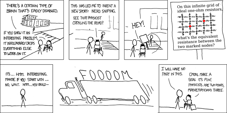
An Instagram ad certianly wasn’t enough to send me down the rabbit hole of topology and complex analysis, but recently, in my math class, we were given the following problem for one point of extra credit.

Can you connect each pair of dots without passing through the box or other connections?

This problem, to me anyways, was tricky! Although I couldn’t find the solution in class, I wanted to try to generalize this problem. What about N points on any surface? Even better, can we write an efficient algorithm to test for the solvability for a generalized connection problem, or perhaps even solve it?

There’s too many questions with not many answers, so let’s dive right in.

Approaching The Puzzle

The first step with any puzzle is to play with it. Let’s try some weirder surfaces and make some observations.

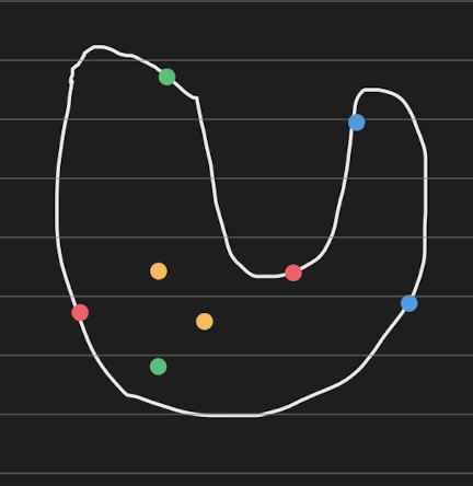
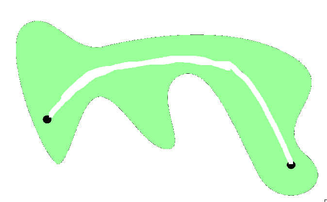
Let’s take a look at this croissant looking shape. There’s a few things to notice here:

• Blue looks awfully easy to connect.
• Yellow looks even easier.
• Dots on the border just look.. plain harder to connect.
• If our croissant looked like this, not much would change.

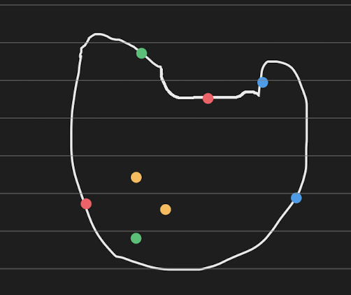
From our recorded observations, there’s two notable takeaways:

• There seems to be a difference between points on the border and points off the border.
• Some changes to the surface don’t change the solvability of the problem.

This inspires a few questions! First, what’s the difference between off and on border point pairs? Does moving a point off or on a border change solvability? What changes to the surface change solvability?

Let’s tackle one at a time. First, let’s look at how different surfaces affect the solvability of the problem.

Surfaces Affecting Solvability

We’ve noticed that there exist ways to modify a surface such that it doesn’t affect the solvability of the problem. It would then follow that we’d need to figure out what modifications to the surface cause a problem set to go from solvable to unsolvable.

The answer, surprisingly, lies deep within the realm of complex analysis. Let’s take a look.

Theorem: If point pairs P are solvable on a proper non-empty simply connected open subset of C, P is solvable on every proper non-empty simply connected open subset of C.

Woah, bold claim, I know. Essentially, what we’re saying is if we can draw the P’s solution on one surface, it implies we can draw P’s solution on any surface! Well, how is this possible?

Let’s make the question more rigorous. What we’re essentially saying is that there exists some transformation from from S1 to S2 such that non-intersecting curves drawn on S1 stay non-intersecting after the transformation. How do we prove this?

Conformal Maps

If you’re familiar with complex analysis, you’ve likely heard of conformal maps. If not, conformal maps are a special type of transformation from one complex set to another complex set such that angles and orientations are preserved. This means two intersecting lines will also intersect at the same angle after the transformation, even if these lines get distorted.

However, there’s absolutely no reason conformal maps need to ensure that non-crossing lines will stay non-crossing. We’d need a new transformation with a slighlty stricter definition to prove this.

Biholomorphic Maps

Enter the biholomorphic map, a specific type of conformal map whose inverse map, the map which reverses the effect of the original map, is also conformal. Let’s try to prove that this transformation will not cross non-crossing lines!

We’ll do this with contradiction. Let’s say we have a biholomorphic map M : A -> B st. A, B e C. Assume M causes non-crossing lines in A to cross in B. It would then follow that M^-1(M(A)) would uncross those lines since A has no crossed lines. However, since M^-1 is a conformal map, crossing lines would need cross at the same angle they were originally intersecting at. Therefore, M cannot cause non-crossing lines in A to cross in B, and as a result cannot cause a problem set to go from solvable to unsolvable! Of course, since M is conformal, it can’t uncross lines either, which means an unsolvable set won’t become solvable after applying M.

Cool! Now that we’ve proved biholomorphic maps don’t change the solvability of a problem set on different surfaces, we just need to prove a biholomorphic map exists between those surfaces. How do we do that?

The Riemann Mapping Theorem

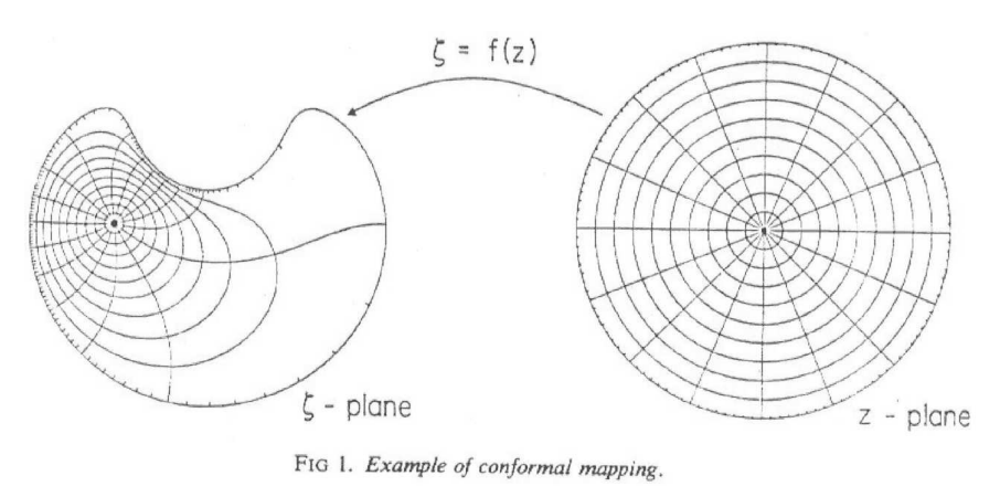
The Riemann mapping theorem states that for every proper non-empty simply connected open subset of the complex plane (what we’ve been calling a surface), there exists a biholomorphic mapping from that subset to the unit disk. Consider the mappings guarenteed by the RMT for both A and B, which we’ll call M_a and M_b respectively. Applying M_b^-1(M_a(A)) will take A to B, without affecting solvability.

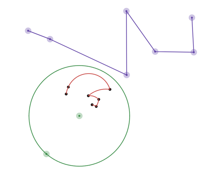
Example of Riemann mapping

Therefore, any problem set solvable on one surface is solvable on every other surface! Pretty neat, huh?

A bit of a nitpick, but RMT only applies to open subsets without a boundary. However, you might have noticed that our surfaces contain points on the boundary, so we need to ensure we have a mapping which includes the boundary. Carathéodory’s theorem tells us that the mapping will still exists as long as the boundary is a Jordan curve. We won’t get into the specifics of Jordan curves until later, but essentialy this means that our boundary must be a closed loop with no self intersection. Since all our surfaces have this property, RMT still applies.

Point Pair Classification

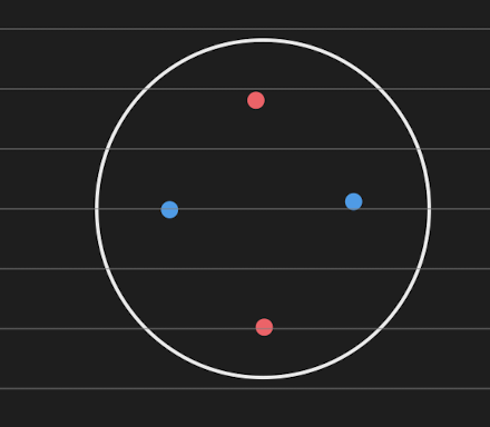
Let’s work on the unit disk now since it’s the simplest surface we can find and play with the different types of point pairs.

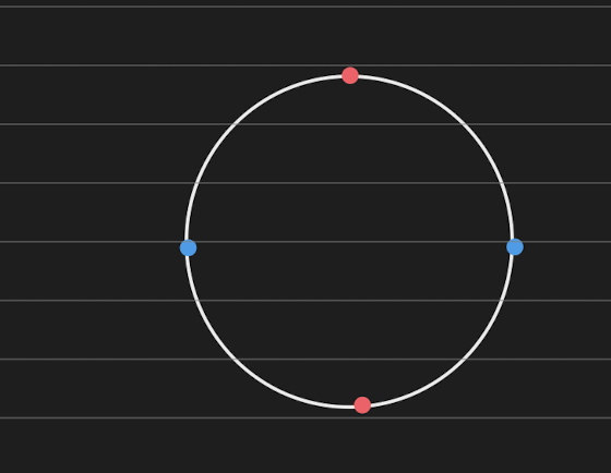
One is clearly solvable, the other isn’t. Well, why? On the first image, all the points are on the border, so it “slices” the circle into two pieces when we connect a pair. How exactly this path is constructed doesn’t really matter, in the end, we end up with two slices.

In the second, the circle isn’t divided at all! When we connect the second pair, we’re able to go around the first pair’s path. This isn’t possible when the points are on the border, since we hit the border of the surface when trying to go around the first path.

Let’s make this property rigorous. We’ll need to classify our point pairs, so lets list them out and give them cute names.

• In the first case, both points in the pair are on the boundary of the surface. Let’s call these points conjoint-conjoint, or CC.
• In the second case, one point is on the surface boundary and the second is off it. Let’s call these points conjoint-disjoint, or CD. Without loss of generality, we can assume that CD = DC, since the point pairs are reflexive.
• In the last case, both points are off the surface boundary. They’ll be called disjoint-disjoint, or DD.

Point Solving with Inversive Geometry & Topology

Allow me to introduce inversive geometry, one of the most powerful tools for solving geometric problems involving circles.

Remember, we solve the problem on the unit disk, we solve it everywhere. However, connecting dots within a circle is kinda hard! If only we could connect the dots on the complex plane, and then map back to the unit disk once we finished.

This is the power of circle inversion, a biholomorphic conformal map that puts everything inside the circle outside the circle and everything outside the circle inside the circle.

If we invert our problem set, solve it on the complex plane, and then invert back, we’ll have solved it on the unit disk!

Point Solving with Path-Connectedness: The Jordan Curve Theorem

It’s time to get into the nitty-gritty: how do we know if our points can be connected?

In topology, there exists the well known property of “path-connectedness”. A “path-connected” space means that there always exists a path between two points on the surface, which we’ll refer to as “spaces”.

This subspace of R² is path-connected, because a path can be drawn between any two points in the space. (Source: Wikipedia)

Although the complex plane is path-connected, what about our case with the outside and inside of the unit circle? Are they path-connected?

Yes! However obvious it seems, we can prove it with the Jordan curve theorem. The Jordan curve theorem states that any Jordan curve, such as the unit circle, divides the space into two seperate spaces, an interior and exterior. These partitions inherit quite a few properties of the original space, one being path-connectedness.

DD Pair Solving: Sutherland’s Path-connected Theorem

This means a DD pair in the exterior of the unit circle will certainly have have a path between them. However, if we had two pairs or a hundred pairs, would drawing one prevent us from connecting the others?

No! We can reframe drawing paths between points on the space as the computing the set difference between the space and the path. All future paths wouldn’t be able to intersect this path, since it’s no longer apart of the space. So, we just need to prove the space remains path-connected after the set difference.

Space with the path removed.

We can use Sutherland’s path-connected theorem to help prove this. It states that connected open subsets of a Euclidean n-space are path-connected. Note that being connected is not the same as being path-connected! One is much harder to prove than the other. Thankfully, we just need to prove the space remains connected after the differences.

Connected Spaces

Spaces are connected if they “cannot be represented as the union of two or more disjoint non-empty open subsets”. If our path divided our spaces into two disjoint spaces, this would cause the space to become disconnected. Because the set is open and the disjoint points are, by definition, finitely spaced from the boundary, the only way for a path to split the set in two would be to create a closed loop. This closed loop, a Jordan curve, by aformentioned Jordan curve theorem, would split our space into an exterior and interior.

However, the path can only be a Jordan curve if the DD points are on top of each other, otherwise there’s no way for the loop to be closed. However, overlapping DD points are already solved, so paths cannot cause the space to go from connected to disconnected!

This means that the space will be path-connected no matter how many DD points we have. In other words, we’ve proved DD points do not affect solvability!

CC Point Solving: Jordan Curve Theorem Returns

Let’s first note that connecting a CC point pair always forms a Jordan curve. By the Jordan curve theorem, there will be an exterior and interior. In addition, the theorem also states any path drawn between a point in the exterior to a point in the interior will intersect the Jordan curve. Essentially, to prove a problem set is solvable, both points in every other pair must be either in the exterior or the interior. A pair cannot straddle the boundary.